by Adrian Worton
Introduction
We are going to look at the years for which batting averages are highest. We will also use the data we find to draw conclusions on individual nations' selection policies. We can also try and look at factors which might bias the data, and we will also have a quick look at normal distributions.
The Data
As there are thousands of test-capped players, we need to sensibly restrict the data. Firstly, time-wise we will only look at players whose careers started after the 1st of January, 1990. This is the same cut-off point as the previous article on averages by opposition. This allows comparisons to be made between the two sets of results.
The second constraint is also for reasons of time: we shall only look at players with at least 50 Test caps. This means that each player will give us plenty of data to work with.
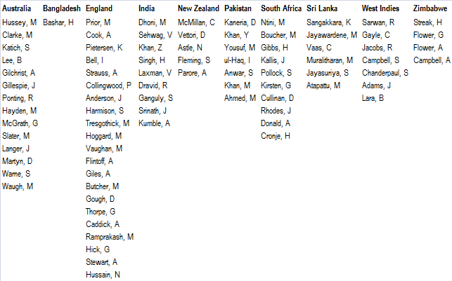
These are the players we ended up with:
As there are thousands of test-capped players, we need to sensibly restrict the data. Firstly, time-wise we will only look at players whose careers started after the 1st of January, 1990. This is the same cut-off point as the previous article on averages by opposition. This allows comparisons to be made between the two sets of results.
The second constraint is also for reasons of time: we shall only look at players with at least 50 Test caps. This means that each player will give us plenty of data to work with.
These are the players we ended up with:
The Method
We then worked out how many runs each player scored in each year of their life, and how many dismissals they had. For each age, we can then add up the total runs made by players at that age, and divide by the total dismissals. We are treating the age a player turns in a particular year as their age for the whole year, as it was far easier to find figures on a calendar-year basis. So if a player was born in (for example) July 1975, then any runs they score in 1995, even if they were before July, count as scored when the player was 20.
The Results
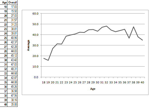
As we are looking at 84 players, over 23 potential years (players in our sample played between ages 18 and 40), then our full data would take up too much space to replicate here. Instead, here is the final averages we got for each age, and their graph:
We then worked out how many runs each player scored in each year of their life, and how many dismissals they had. For each age, we can then add up the total runs made by players at that age, and divide by the total dismissals. We are treating the age a player turns in a particular year as their age for the whole year, as it was far easier to find figures on a calendar-year basis. So if a player was born in (for example) July 1975, then any runs they score in 1995, even if they were before July, count as scored when the player was 20.
The Results
As we are looking at 84 players, over 23 potential years (players in our sample played between ages 18 and 40), then our full data would take up too much space to replicate here. Instead, here is the final averages we got for each age, and their graph:
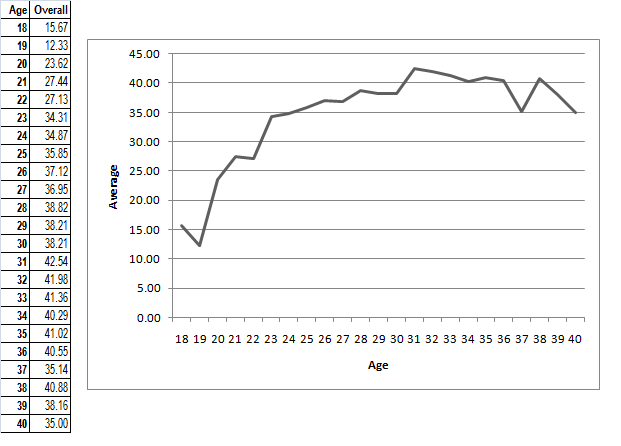
Firstly, we can see that the age with the highest average is 31. We can see that averages are generally lower in the 20's than they are throughout the 30's. And finally, the data is far more variable around the extremes of our data (18-20 & 37-40).
Influences on the Data
Quality - is our data skewed in any way by the fact we only chose players with at least 50 caps? These generally will be the best players from their nation over the time period, otherwise they wouldn't have been chosen so often. Therefore we can expect their batting averages to be higher than the norm. However, there is no indication whether they would have an effect on a particular age range more than others. So we cannot categorically state how this affects the data without running the same tests with no restrictions on caps.
Quantity - we have 84 players in our database, with over 10,000 dismissals between them. However, as we've discovered, players seemingly peak in their early 30's, so those players are more likely to be chosen. The graph below shows how many players we have in our database for each age:
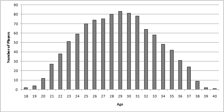
Now we can see why our data was more variable around the edges - there is far less data to work with. So it might be sensible to only consider the data between ages 21 - 37. This does not really change our conclusions. We will discuss the shape of this graph later.
Bowlers - one influence on our data, which might pose a problem with biasing the results is the impact of bowlers. It is generally considered that fast bowlers' careers are over quicker than spin bowlers and batsmen. This is due to the physical exertions they have to go through, as well as they rely a lot on their physical attibutes. This is why the highest wicket-takers in Test history are spin bowlers.
Naturally, a player who is a specialist bowler will generally have a lower batting average than a specialist batsman (especially the calibre of batsmen on our list). Therefore if we have a group of players dragging down the average for only the earlier years, then this affects our data. Therefore we decided to try and take this into account. However, rather than looking at each individual player and working out their role (for instance, looking at whether certain players are batting all-rounders, or bowling all-rounders), we decided to exclude all players with an average below 25.00. Those results were:
As we antitipated, the data for players in their 20's rises. However, there is also the unexpected consequence in that our new peak year is 32. Rather than a peak of the early 30s, it is now restricted to just the ages of 31 and 30. As with before, our data is highly variable around the fringes, presumerably because there's even less data to work with.
Normal Distributions
Normal Distributions
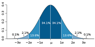
Anyone who has studied statistics will recognise the graph of numbers of players per age as something approximating a normal distribution, also known as a bell-curve, pictured left.
The calculations behind the normal curve are a little complicated to explain here, but it turns out it is a very good approximation of how a lot of real-life data is distributed, from the heights of people to the lengths of songs. In the diagram to the left, σ (sigma) represents the standard deviation of the data, and μ (mu) is the mean. If you have the mean and standard deviation of a set of data, it can be easily modelled as a normal distribution.
Individual Teams
It would be a waste not to use the information we've collected and use it to look at individual nations. First of all, we will look at the number of players on the list. On the graph below you can see (in blue) how many players each team contributed to our list, and in red you can see how many matches each team has played from 1990 onwards. On average, teams played 20 more games than they had players with over 50 caps, so we divided the amount of games by 20.
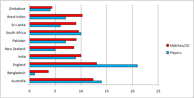
The only nation which has considerably more than 1 player to reach 50 caps per 20 games is England. The ones which are considerably below are the West Indies, New Zealand, Sri Lanka and Bangladesh. These nations all at some stage over the 22 years were quite weak, so perhaps they have so few players good enough to merit 50 caps. Bangladesh have only had about a decade to get players up to 50 caps.
However, this argument does not extend to England - they were very poor during the 1990s, yet have a huge amount of players with over 50 caps. This seems to indicate that England tend to stick with players for a medium duration of games, before giving someone a turn. This indicates that perhaps they are too slow to replace poor players.
Much more understandably, the two most successful Test nations during this period, Australia and South Africa, have the most players with over 50 caps.
We can also look at the average age of players in our database. This is inexact, as it's unlikely that 18 year-old players play as many games per year as a 30 year-old, however it still allows us to compare the different nations. We have excluded Bangladesh as they only have one player in the list. Here is the result:
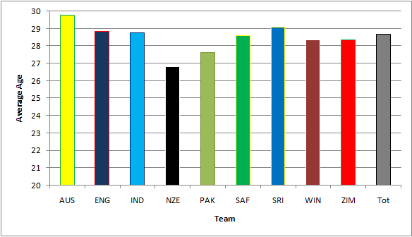
The only especially interesting nations here are Australia and New Zealand, at each extreme. Australia is not particularly surprising, they had a golden age in the 90s, so it's not surprising they stuck with those players, stretching the average upwards. New Zealand have struggled over the time period, after a few key players retired at the start of the 90s, so have been struggling to find the right new players.
What is interesting to note is that every team's average is below 30, with only Australia and Sri Lanka above 29. As we've discovered, the peak for batsmen is between 31 and 32, so perhaps some teams need to try older batsmen in order to gain an advantage.
Conclusion
We've found that batsmen peak around the ages of 31-32. We also saw that fast bowlers skew the data due to their earlier retirements. Most satisfyingly, we also saw that the age of batsmen is a very close approximation to a normal distribution.
Sources
Statsguru - used for collecting career statistics of our players.
Wikipedia - this link will take you to an article on the bean machine. This was invented over 100 years ago as a way of demonstrating the normal distribution in action. Wikipedia was also used to find which cricketers had over 50 caps, and for the diagram of the normal distribution used above.
 RSS Feed